S-Band FMCW Radar with MIMO Antenna Array Beamforming

FMCW MIMO Array Calibration

The k-th time discrete IF signal of an ideal point target of the proposed FMCW radar can be represented with equations 2, 3 and 4 [8]. It is a sine wave with the amplitude a0 defined by the reflectivity and distance of the target and frequency f^IF_k and phase ϕ^IF_k depending on the distance of the target to each Tx/Rx antenna combination. The parameter µ is the frequency ramp speed defined by the bandwidth divided by the ramp pulse time. f₁ is the ramp start frequency.

Matchmaker+ Anbieter zum Thema

zu Matchmaker+

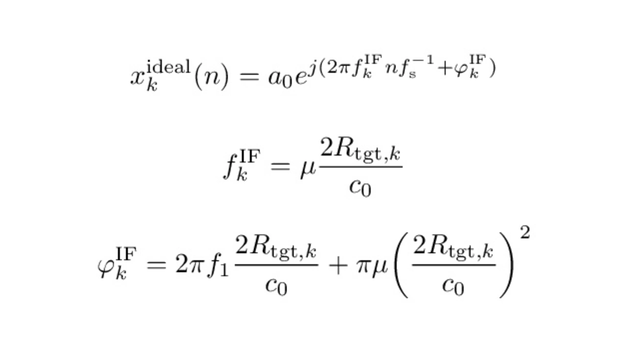
The last term in equation 4 is referred as residual video phase error (RVP) and can be corrected by a range deskew algorithm or in case of the proposed radar in this paper can be discarded due to negligible influence [9].

Parasitic phenomena are present in a MIMO FMCW radar in practice, that makes a prior calibration of the raw signals necessary [2]. First, phase offsets are present, for example due to different lengths of RF cables to the antennas or in the local oscillator signal distribution. These length offsets can exceed several phase shifts of over 2π and then result in a frequency shift, such that a target lies in different range bins for each virtual antenna channel.

Second, each channel has different gain characteristics. These amplitude characteristics are not only different from channel to channel, but also varies over frequency or in case of an FMCW radar over the pulse time. The amplitude response needs to be corrected by the calibration algorithm, otherwise it would result in an amplitude modulation and the target peak could be spread out or ghost targets could appear.

Furthermore, phase nonlinearities of the rf components lead to a phase modulation of the beat signals and can also decrease the resolution of the radar, respectively can lead to the generation of ghost targets.

Calibration Method

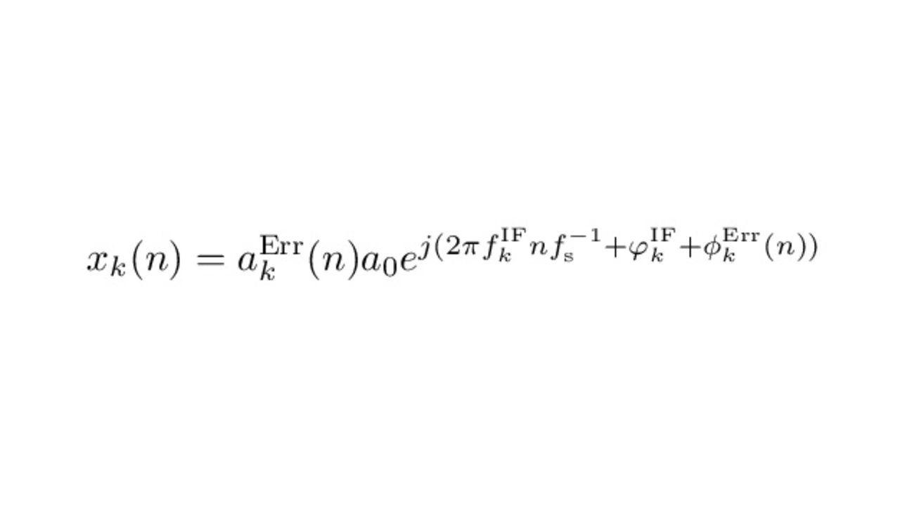
The error containing IF signal is modeled in equation 5, where a^Err_k(n) is the time dependent amplitude error and ϕ^Err_k(n) the time dependent phase error, containing phase nonlinearities and frequency offsets.

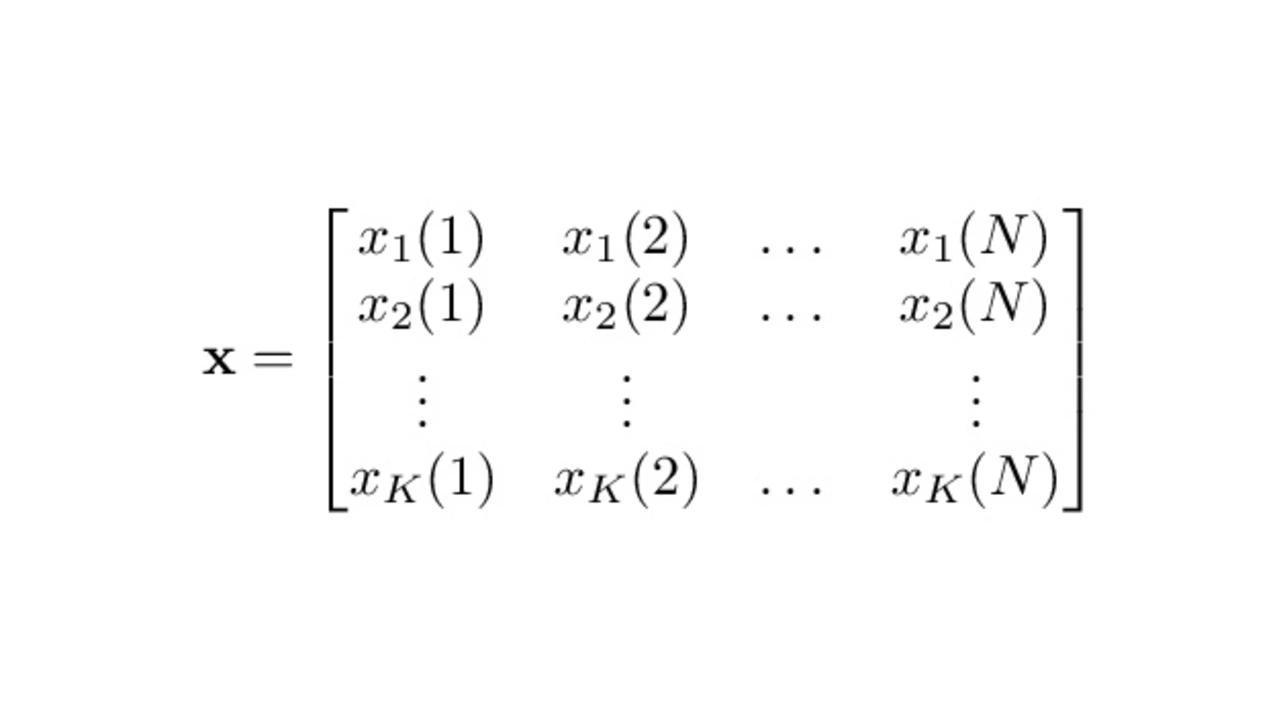
The uncalibrated sample matrix in equation 6 is of size K×N and contains the N time samples of all K virtual antenna channels, including the error terms.

To calibrate the sample matrix, it is multiplied with a calibration matrix s_cal. The calibration matrix is gathered in four following steps:

1. Measure the sample matrix x of a strong target in the boresight of the radar (incident angle ϴ = 0°).
2. Calculate the DFT (Discrete Fourier Transformation) of the time signals of every virtual antenna channel. One can use zero-padding to increase the range accuracy.
3. Window the signals at each target peak with a rectangular window. The width should be chosen, such that the target response lies inside the window. In this work the width was between 1 m and 2 m.
4. Calculate the inverse DFT of the windowed signals to gather x_windowed.

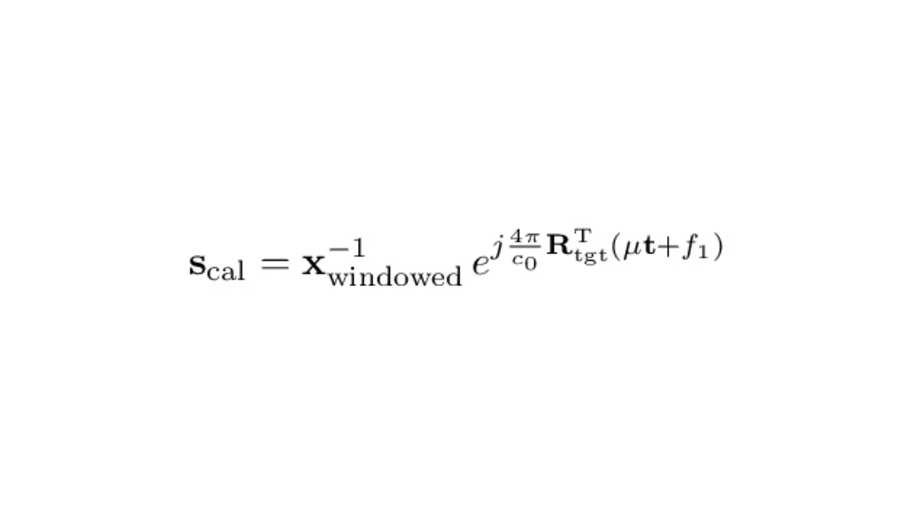
The windowed target response x_windowed is then used to calculate the calibration matrix s_cal. Target peak windowing makes sure, that no unwanted clutter effects the calculation of the calibration matrix and also noise is filtered out from unwanted range bins. The calculation of s_cal is shown in equation 7. The inverse of the windowed measured sample matrix is taken and then multiplied with the theoretical expected time signal which is given in equation 2, 3 and 4.

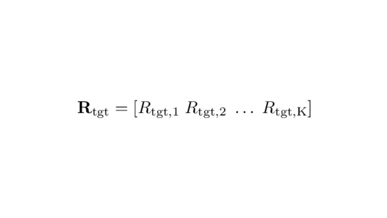
Because in a realistic environment, the distance to the calibration target is limited, as in our case to a few meters, the reflected wave is not a perfect plane wave anymore. Instead the reflected wavefront arrives in a spherical shape across the array, this is accounted by considering each distance from the virtual antenna to the target. Therefore, a target distance vector is introduced with equation 8.

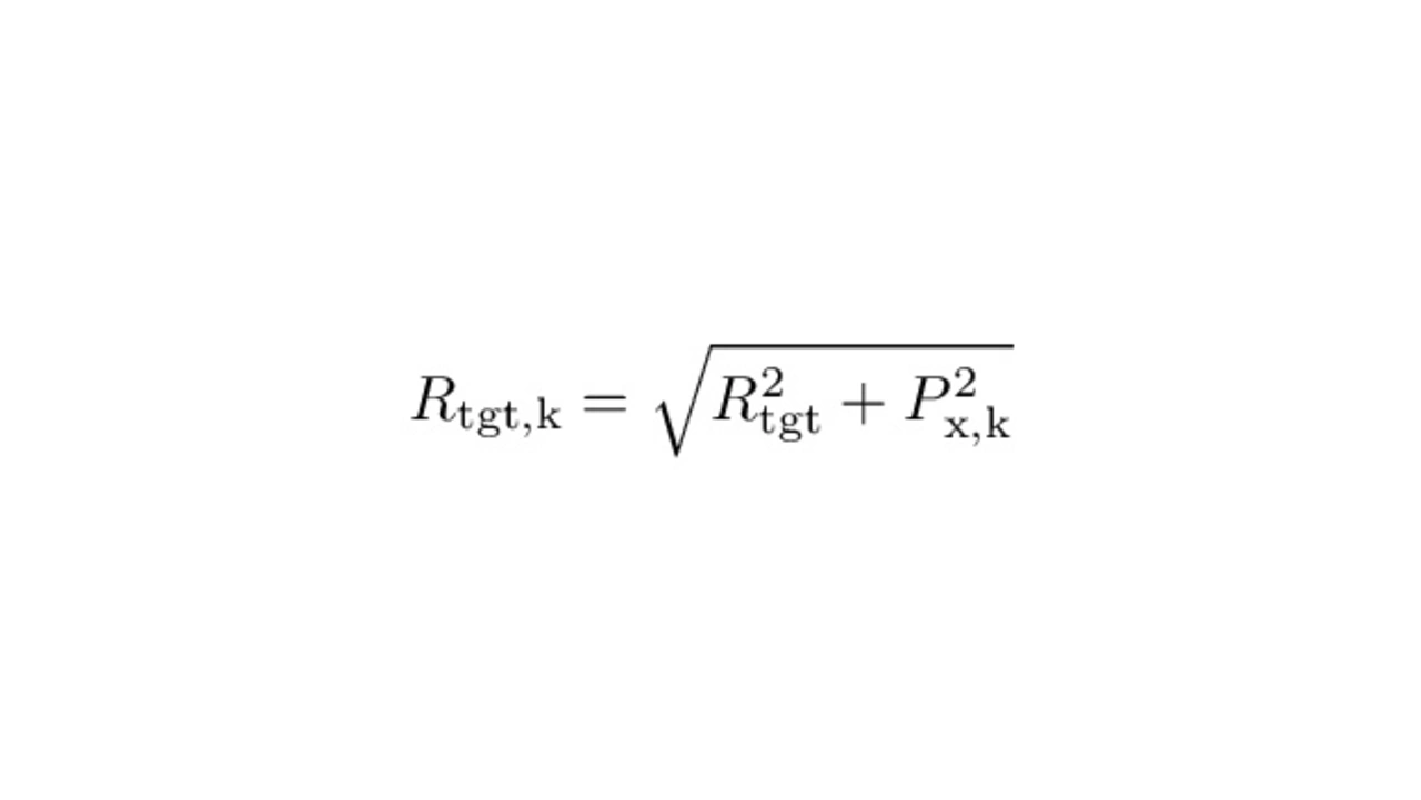
The target distance vector for a target that lies exactly boresight to the radar, that is perpendicular and in the center of the array-axis, can be calculated with equation 9. Where R_tgt is the shortest distance from the ULA to the target and P_x,k is the k-th ULA antenna position on the x-axis.

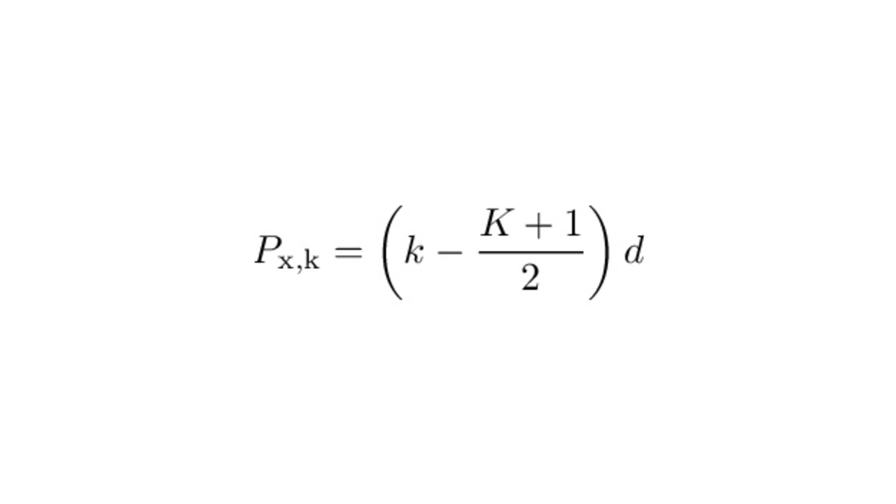
The antenna positions Px,k for a ULA can be calculated with equation 10.

Properties of Calibration Matrix

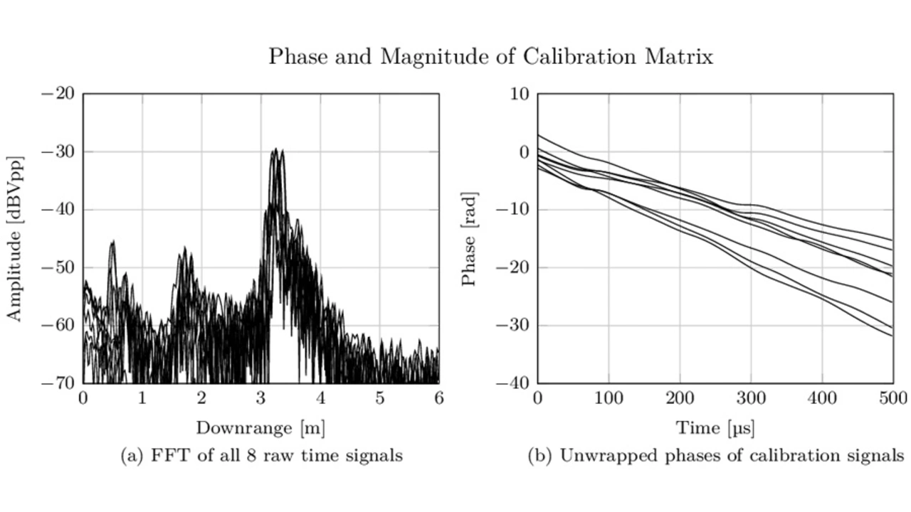
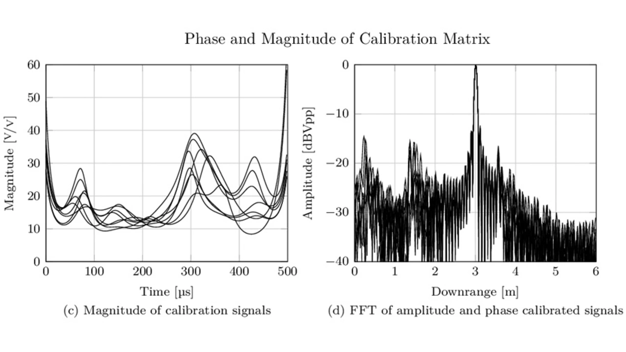
Figure 6 shows the magnitude and phase of the time signals in the calibration matrix as well as a measurement of a dihedral corner reflector at a distance of 3 m boresight to the radar. Plot (a) shows the uncalibrated range plots of all eight virtual antenna channels. The target peak lies in different range bins and the peak itself is spread due to slight phase nonlinearities and amplitude distortions. Plot (b) shows the unwrapped phase of the calibration signals, the constant linear slope equals frequency offsets due to different cable lengths and variations from these constant slopes are due to phase nonlinearities. Plot (c) shows the magnitude of the calibration signals. In plot (d) is the range plot of the calibrated sample matrix. The target peak lies now in the same range bin and looks much cleaner.

Results

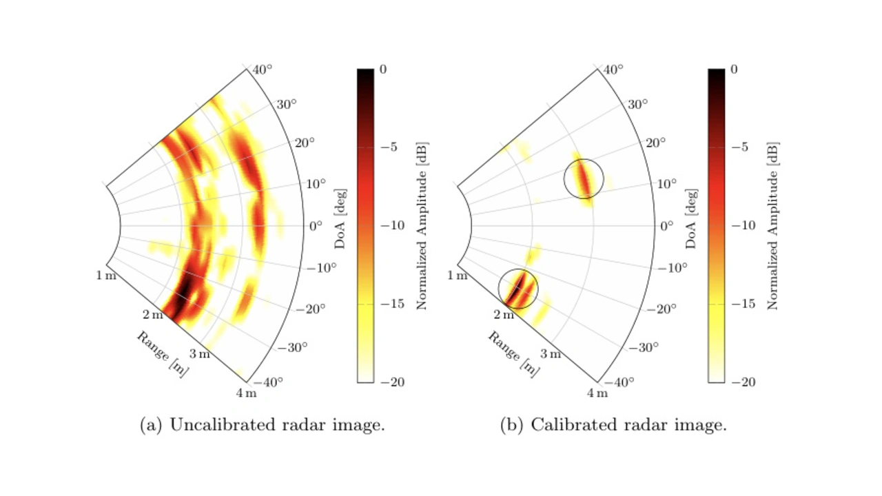
Two radar images of the same scene are shown in figure 7. The scene consists of two targets, a dihedral corner reflector at a distance of 2 m and at an angle of -30° and a trihedral reflector at 3 m and 15°. In subfigure (a), the image was created with a 2-dimensional DFT of the raw radar data. In subfigure (b), the raw radar data was first calibrated using the proposed calibration procedure and the image was then reconstructed using the 2-dimensional DFT.

The image in subfigure (a) is blurred in the DoA (Direction of Arrival) domain as well as in the range domain due to parasitic effects discussed in the sections before. Whereas, the targets shown in the calibrated image (b) are well localizable. The parasitic effects have been eliminated due to the calibration prior to the image processing.

Bibliography

[1] Davis, M.: Foliage penetration Radar: Detection and characterisation of objects under trees. 01 2011.

[2] Frischen, A.;  Hasch, J. and Waldschmidt, C.: Fmcw ramp non-linearity effects and measurement technique for cooperative radar. European Radar Conference (EuRAD), 2015, pp. 509–512.

[3] Hong J. and Lancaster, M.: Microstrip Filters for RF / Microwave Applications. Wiley Series in Microwave and Optical Engineering, 2004.

[4] Nurhayati, N.; Setijadi, E. and Hendrantoro, G.: Radiation pattern analysis and modelling of coplanar vivaldi antenna element for linear array pattern evaluation. Progress In Electromagnetics Research B, 2019, vol. 84, pp. 79–96.

[5] Ukaegbu I. and Gamage, K.: Parametric analysis and bandwidth optimization of hybrid linear-exponential tapered slot vivaldi antennas. Loughborough Antennas & Propagation Conference (LAPC 2017) 2017, pp. 55–59.

[6] Trees, H. L. V.: Optimum Array Processing: Part IV of Detection, Estimation, and Modulation Theory. Wiley, 2002.

[7] Sun, H.; Brigui, F. and Lesturgie, M.: Analysis and comparison of mimo radar waveforms. International Radar Conference 2014

[8] Gardill, M.: Characterization and design of small array antennas for direction-of-arrival estimation for ultra-wideband industrial fmcw radar systems. Doctoralthesis, FAU University Press, 2015.

[9] Carrar, W.; Goodman, R. and Majewski, R.: Spotlight Synthetic Aperture Radar: Signal Processing Algorithms. Artech House Remote Sensing Library, 1995.

The authors

Maximilian Sundermeier. M. Sc.

studied electronics with the focus at microwaves and communication systems at the University of Applied Sciences Münster. He graduated with a master's degree in 2019 at the DLR in Oberpfaffenhofen. Since 2019, he is a PhD student at the University of Applied Sciences Münster in cooperation with the TU Chemnitz.

max.sundermeier@fh-muenster.de

Prof. Dr.-Ing. Dirk Fischer

studied electronics from 1986 to 1991 at the TU in Dortmund, subsequently he graduated with a PhD in the region of optical communications at the TU Dortmund. He worked as a microwave engineer until 1999 and works since 2000 as a Professor at the University of Applied Sciences Münster.

dirk.fischer@fh-muenster.de

1. S-Band FMCW Radar with MIMO Antenna Array Beamforming
2. FMCW MIMO Array Calibration